
Curious about how to make a drop down list in Excel? And why you would want a drop down list?Read on…
First–why would you want to use a drop down list?
- Quality control. If you limit the choices you can ensure that incorrect data will not be entered, particularly if you handle the error messages correctly — more on that later.
- Efficiency. If users have a menu presented, their data entry is simplified and streamlined.
- Instruction. Using the optional messages available, you can train users.
Hopefully, this is enough to sell you on using a drop down lists. Now we will tackle how to create a list.
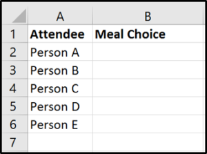
Hypothetical situation: you are tracking the meal choices of attendees at a conference. The options are: Steak, Chicken, Fish, Vegetarian, Vegan.
You need to sort the attendees by their meal choice for the caterer, but you don’t want misspellings or entries that are not allowed (e.g. pasta or eggs).
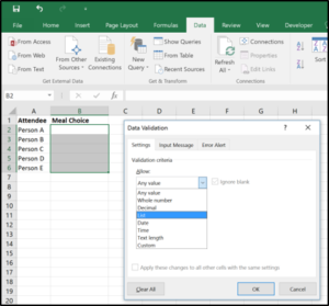
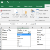
Select the cells where you want the drop down list to appear. Go to the Data tab, and choose Data Validation. (Why is it called Data Validation? By limiting the choices that can be entered, you are validating the data that is entered.)

Once the Data Validation dialogue box appears, choose List in the Allow field. (Yes, there are lots of other types of data validation, and in future posts, I will explore those too. )
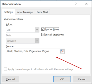
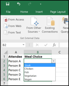
Enter the list directly in the Source field. This is a great option for short lists (3-5 choices). Separate the choices by commas. Click OK and you have a drop down list.
But what if you have a much longer list? Or a list that is already created elsewhere in the workbook or even in another workbook? Easy. In the picture below, you see that I have created a list in the cells D1 through D7. (These cells happen to be on the same worksheet, but they don’t have to be.)
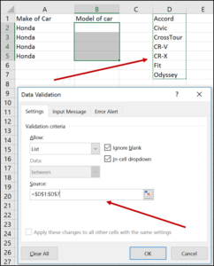
In the Source field, enter the cell names with the “=” sign in front of them. Also, be sure to enter a dollar sign in front of both the column name and the row name–as in the example. (In a future post, I will talk about the dollar signs, and what they mean in Excel.) Alternatively, you can select the cells that contain your list, and Excel will auto-populate it for you.
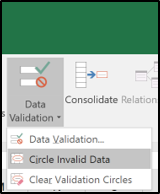
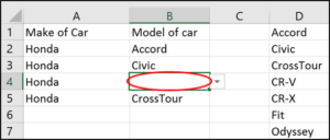
Now let’s do some fine tuning. The default for a drop down list is to ‘ignore blanks’. Go back and look at one of the screenshots–you will see a check box that is defaulted to checked. Unchecking that box does nothing during the data entry process. However, if you want to find all the ‘invalid data’ data cells with data validation, you can use the Circle Invalid Data option under the Data Validation menu.
On Friday, I will talk about how to create useful messages to help users navigate your data validation.
In the meantime, keep soaring.